

Can Margin Debt Assist Predict SPY’s Progress & Bear Markets?
Navigating the monetary markets requires a eager understanding of danger sentiment, and one often-overlooked dataset that gives worthwhile insights is FINRA’s margin debt statistics. Reported month-to-month, these figures observe the overall debit balances in prospects’ securities margin accounts—a key proxy for speculative exercise out there. Since margin accounts are closely used for leveraged trades, shifts in margin debt ranges can sign adjustments in total danger urge for food. Our analysis explores how this dataset could be leveraged as a market timing device for US inventory indexes, enhancing conventional trend-following methods that rely solely on value motion. Given the present uncertainty surrounding Trump’s presidency, margin debt information might function a warning system, serving to buyers distinguish between market corrections and deeper bear markets.
Borrowing to speculate is a typical technique that may amplify each returns and dangers in monetary markets. One key measure of this leverage is margin debt—the overall quantity buyers borrow to purchase shares utilizing their holdings as collateral. A rise in margin debt usually alerts rising investor confidence and a willingness to tackle extra danger, which might drive inventory costs increased. Conversely, a decline in margin debt could point out danger aversion, deleveraging, or market uncertainty, doubtlessly resulting in decrease inventory costs. Given its robust connection to market sentiment and liquidity, margin debt can function a worthwhile indicator of inventory market actions. Subsequently, our purpose is to discover how margin debt could be utilized to foretell SPY value development by growing a scientific funding technique.
FINRA was the supply for margin debt information, and information could be simply obtained beginning in 1998. Subsequently, we used SPY as a proxy for the inventory market efficiency from January 30, 1998, to December 31, 2024. FINRA studies margin debt statistics month-to-month, so all calculations on this article are based mostly on month-to-month information, and every particular person examined technique was rebalanced month-to-month, too.
Methodology
Much like our earlier market timing research (like Utilizing Inflation Information for Systematic Gold and Treasury Funding Methods or Insights from the Geopolitical Sentiment Index made with Google Traits), we aimed firstly to know the conduct of the brand new information set and visualization of the dataset helps with that:
Visible evaluation uncovers that the native peaks in margin debt appear to coincide in time with the native peaks within the SPY; nonetheless, every so often, the margin debt peaks precede the SPY peaks by a couple of months. The inventory market indexes are well-known for his or her trending conduct, and trend-following guidelines work effectively on indexes. Subsequently, our subsequent step was to attempt to use comparable trend-following guidelines additionally for the margin debt dataset and research whether or not the alerts from the margin debt information outperform price-based alerts alone, alternatively, whether or not we are able to mix value and margin debt alerts to acquire methods with higher efficiency of return-to-risk rations then pure price-based development methods.
As we wish to evaluate the margin debt alerts (and the mix of value + margin debt alerts) to price-based methods, we first should research these price-based development methods to create a benchmark that we are going to then attempt to beat.
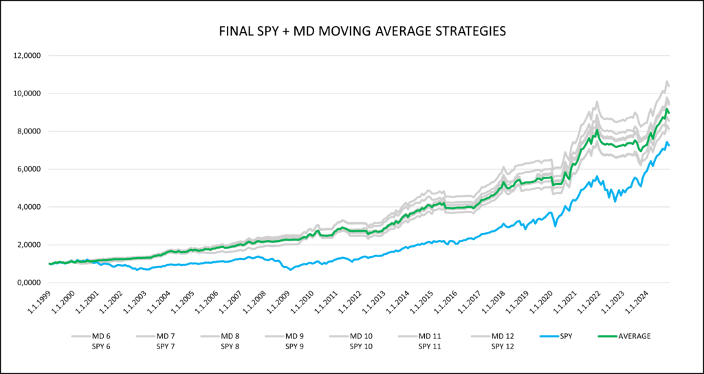
Our default “go to” price-based predictor for SPY is normally a easy transferring common. We started with a 3-month transferring common and progressively elevated the window to 4, then 5 months, persevering with this course of till we reached a 12-month transferring common of SPY complete return (dividend & split-adjusted) value collection (normalized to begin at 1$ on January 30, 1998). On the finish of every month, the latest accessible worth was in comparison with the transferring common. If the newest SPY worth exceeded the transferring common, it signaled a SPY lengthy place for the subsequent month. In any other case, we assumed that as a substitute of investing in a dangerous asset (SPY ETF), capital can be held in a low-risk asset represented by SHY ETF (iShares 1-3 12 months Treasury Bond ETF, a typical proxy for the low-risk, cash-like funding). This process was utilized to every transferring common interval. To find out how every development technique with every transferring common interval of SPY fared, we additionally visually in contrast particular person methods, following the strategy utilized in Easy methods to Enhance Commodity Momentum Utilizing Intra-Market Correlation. For higher perception, each month, the common of all transferring averages was calculated to acquire the equally weighted common technique throughout every transferring common. This “common trend-following technique” is our proxy for the benchmark, and we want to beat it with the utilization of the margin debt information.
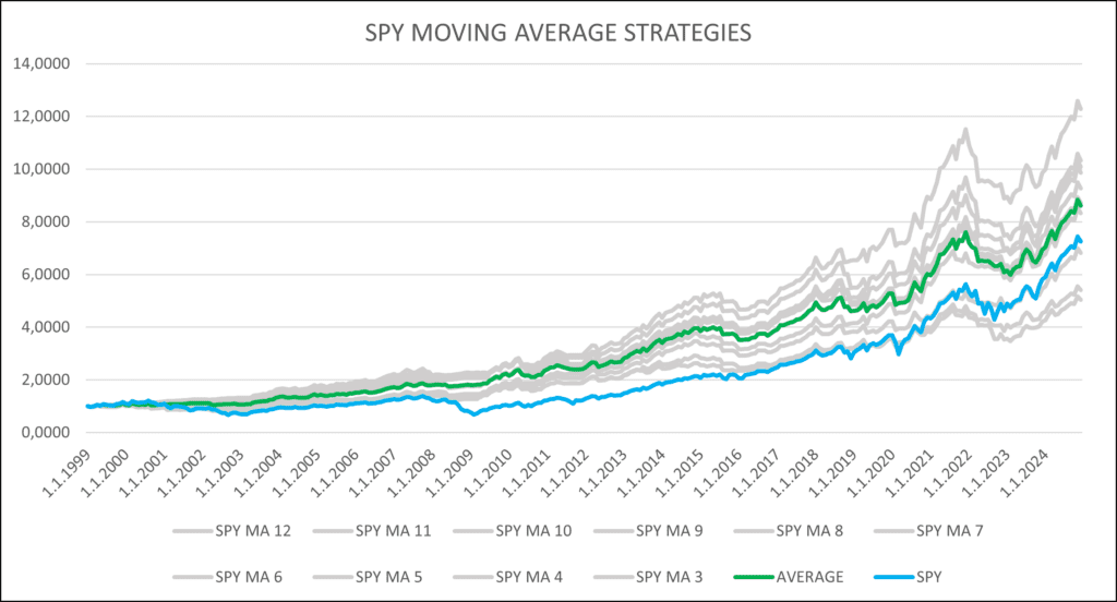

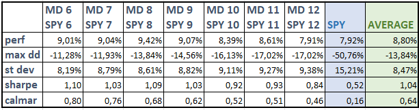
Each numerical calculations and visible illustrations point out that SPY’s transferring averages are efficient predictors for SPY itself. The methods utilizing tendencies with medium size (6-12 months) all beat SPY on the efficiency foundation and return-to-risk foundation. Despite the fact that the efficiency of methods utilizing the 3-, 4-, and 5-month transferring averages are decrease than SPY’s, their commonplace deviation or most drawdown is considerably decrease than SPY’s and, due to this fact, have increased Sharpe and Calmar ratios. The typical of all the development methods additionally outperforms SPY in all points (efficiency and return-to-risk measures, too).
Nonetheless, this isn’t a brand new reality. What pursuits us, nonetheless, is how methods based mostly on margin debt information will carry out as compared… Will they be capable to obtain higher outcomes?
To find out whether or not the transferring common of margin debt is a greater predictor for SPY than its personal transferring common of value, we repeated the identical process and created methods based mostly on 10 totally different transferring averages of margin debt (3-month, 4-month, …, 12-month transferring averages). We additionally constructed an equally weighted technique combining these transferring averages and in contrast their efficiency to SPY’s efficiency.
The testing precept stays the identical: when the newest accessible margin debt worth was increased than its transferring common, we purchased SPY. In any other case, the capital was held in money. Nonetheless, margin debt information is usually launched with a one-month lag, that means the purchase sign relies on month-old values, in contrast to SPY’s transferring averages, which use real-time costs. So, for instance, for a transferring common calculation of the SPY on the finish of Could, we are able to use the value information from the top of Could (as they’re recognized on a tick-by-tick, second-to-second, minute-to-minute foundation). Then again, once we calculate the transferring common sign from the margin debt information, we use April because the final information level for the calculation on the finish of Could, as FINRA normally distributes April’s information within the second half of Could and extra updated information are usually not accessible at the moment.
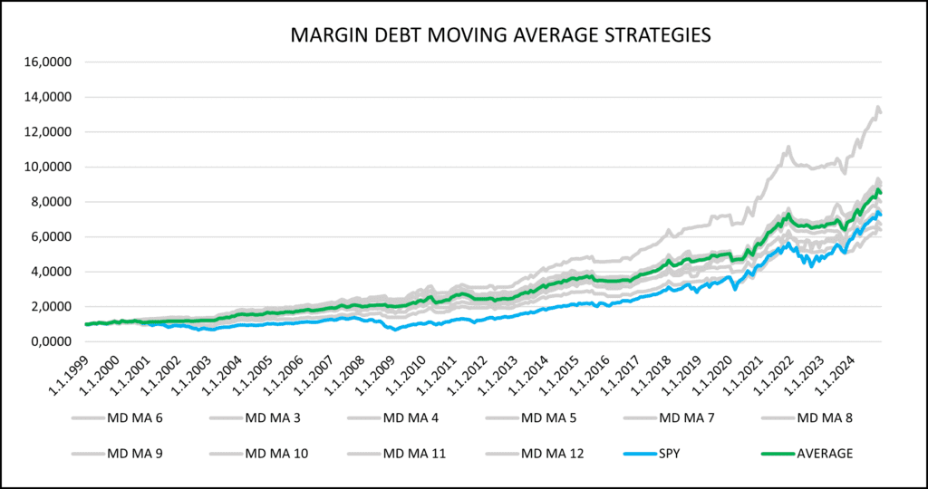

At first look, there aren’t any clear visible variations between the fairness curves in Determine 2 and Determine 3. Subsequently, numerical traits are extra informative. On common, return-to-risk measures from Desk 2 (methods utilizing margin debt information) exceed return-to-risk ratio measures of methods based mostly on value transferring averages alone. Subsequently, we are able to conclude that, throughout our pattern, the margin debt methods have certainly profitably predicted SPY’s conduct. Nonetheless, the value motion of SPY itself can also be a good predictor. Subsequently, within the subsequent half, we’ll mix these two predictors into one technique.
On this step, we determined to mix the 2 earlier methods and asses whether or not the mixed technique has higher market timing traits and outperforms particular person parts alone. Every transferring common interval of SPY was assigned the corresponding transferring common of margin debt for a similar interval. If the final accessible information level of each information collection have been increased than their respective transferring averages on the identical time, we acquired a sign to put money into SPY. In any other case, the capital was held within the risk-free asset (SHY ETF).
With this strategy, we created 10 new indicators, the 3-month transferring common of SPY mixed with the 3-month transferring common of margin debt, …, as much as the 12-month transferring averages of each. Equally weighted (common) technique of transferring common pairs was additionally constructed. As soon as once more, margin debt costs have been lagged by one month, whereas SPY costs have been updated at any given time.
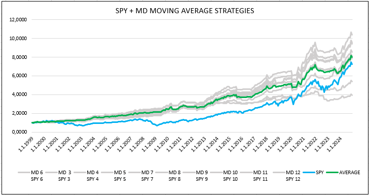
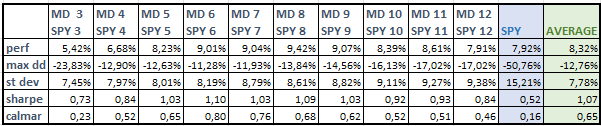
Now, we are able to evaluate the ends in Desk 3 (mixed technique) with particular person predictors in Tables 1 & 2. On common, the return-to-risk measures of the mixed methods are increased than these of particular person parts, and this holds true primarily for the medium-term, 6-12-month horizons.
If we assessment the fairness curves of the mixed methods, we are able to see that over the past three years of the testing interval, SPY achieved increased returns than some mixed methods. In Desk 1 and Desk 2, we are able to see that transferring averages for shorter durations, particularly 3-, 4-, and 5-month durations, achieved decrease returns than the longer ones (6-12 months). This may be only a non permanent setback, or it might probably counsel that longer time-frames (6-12 months) are higher suited as predictors for the underlying datasets. The 6- to 12-month interval can also be probably the most used interval for trend-following predictors within the educational literature. Because of this, we determined to exclude 3- to 5-month interval from our remaining mannequin.
The typical technique is now designed so that each month capital is equally distributed throughout seven methods utilizing the mixed transferring averages (the 6-month transferring common of SPY mixed with the 6-month transferring common of margin debt, …, as much as the 12-month transferring averages of each).
The thought of not constructing the ultimate technique on only one finest parameter (for instance, 8-month transferring common), however averaging over extra parameters can also be supported by our findings from our older article – Easy methods to Select the Finest Interval for Indicators. Our evaluation means that as a substitute of counting on a single indicator, a set of a number of indicators with totally different durations needs to be used, as this strategy reduces the chance of underperformance in future durations. If one indicator doesn’t carry out effectively within the out-of-sample interval, the others can compensate for its weak efficiency.
Earlier than we conclude, we could ask another query – Why not mix the perfect transferring common interval of margin debt with the perfect interval of the SPY’s transferring common? As proven in Determine 3, the 6-month transferring common of margin debt achieved considerably increased returns (and return-to-risk ratios) than different parameters. Nonetheless, we consider that this incidence is only a stroke of luck and won’t be sustained sooner or later, and ultimately, imply reversion will happen. Subsequently, as soon as once more, we choose to unfold out bets within the portfolio amongst all the different parameters to have a extra steady mannequin.
Conclusion
Our expectations have been met— the margin debt dataset can certainly be used to foretell SPY’s value development. Whereas the transferring common of SPY alone serves as a powerful indicator, combining it with the transferring common of margin debt additional enhances its predictive energy. This impact is most pronounced for transferring averages with lengths between 6 and 12 months. The optimum strategy for mitigating the affect of potential future imply reversion in returns is to distribute investments equally throughout a number of durations of those mixed trend-following methods and make sure that if the efficiency of 1 explicit transferring common interval declines, the others might help maintain total profitability.
Writer: Sona Beluska, Quant Analyst, Quantpedia
Are you searching for extra methods to examine? Join our publication or go to our Weblog or Screener.
Do you wish to study extra about Quantpedia Premium service? Examine how Quantpedia works, our mission and Premium pricing supply.
Do you wish to study extra about Quantpedia Professional service? Examine its description, watch movies, assessment reporting capabilities and go to our pricing supply.
Are you searching for historic information or backtesting platforms? Examine our listing of Algo Buying and selling Reductions.
Or observe us on:
Fb Group, Fb Web page, Twitter, Bluesky, Linkedin, Medium or Youtube
Share onLinkedInTwitterFacebookDiscuss with a buddy


